Excel is a powerful tool for analyzing data, and one of its most basic functions is calculating the average of a set of numbers. In this post, we’ll explore three different ways to find the average in Excel: using the average function, the averageif function, and the subtotal function with the average function. We’ll also highlight how the subtotal function can help you calculate the average only for the visible rows, making it ideal for working with filtered data.
Using the Average Function
The average function is the most straightforward way to find the average of a set of numbers in Excel. To use it, simply follow these steps:
1. Select the cell where you want to display the average.
2. Enter the formula “=AVERAGE(range)”, where “range” is the range of cells you want to average.
3. Press Enter
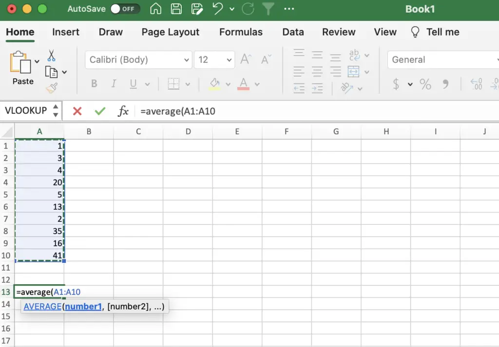
For example, if you want to find the average of the numbers in cells A1 through A10, you would enter “=AVERAGE(A1:A10)” in the cell where you want to display the result.

Using the Averageif Function
The averageif function allows you to find the average of a range of cells that meet a specific condition. To use it, follow these steps:
1. Select the cell where you want to display the average.
2. Enter the formula “=AVERAGEIF(range, criteria, average_range)”, where “range” is the range of cells you want to evaluate, “criteria” is the condition you want to apply, and “average_range” is the range of cells you want to average.
3. Press Enter.
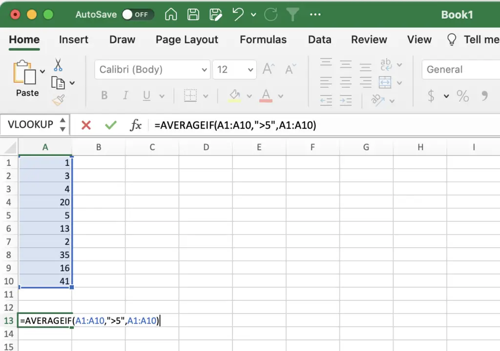
For example, if you want to find the average of the numbers in cells A1 through A10 that are greater than 5, you would enter “=AVERAGEIF(A1:A10,”>5″,A1:A10)” in the cell where you want to display the result.

Using the Subtotal Function with Average
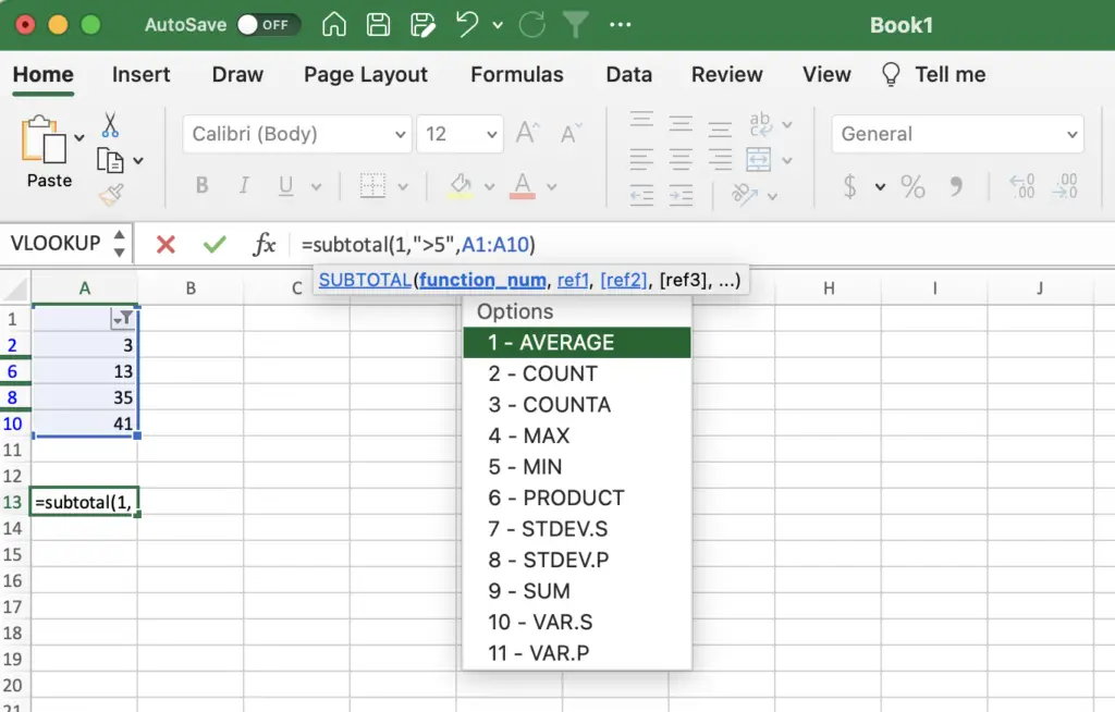
The subtotal function allows you to perform calculations on a subset of data, such as the visible rows in a filtered table. To use it with the average function, follow these steps:
1. Select the cell where you want to display the average.
2. Enter the formula “=SUBTOTAL(1,range)/SUBTOTAL(103,range)”, where “range” is the range of cells you want to average.
3. Press Enter.
The first part of the formula, “=SUBTOTAL(1,range)”, calculates the sum of the visible cells in the range. The second part, “/SUBTOTAL(103,range)”, counts the number of visible cells in the range. Dividing the sum by the count gives you the average of the visible cells.
For example, if you want to find the average of the visible numbers in cells A1 through A10 after filtering the table, you would enter “=SUBTOTAL(1,A1:A10)/SUBTOTAL(103,A1:A10)” in the cell where you want to display the result.

Conclusion
Calculating the average of a set of numbers is a basic but essential function in Excel. Whether you’re using the average function, the averageif function, or the subtotal function, Excel has the flexibility to help you average numbers in an efficient and effective manner!